Joins Algorithms
在 RDBMS 中,我們常常會依據正規化 (normalization) 的原則將資料放到不同的表格中以避免記錄到重複的資料,因此在查詢時,我們就需要透過 join 來將資料合併。
在這篇筆記中,我們主要會討論兩個 table 執行 join 的不同方法。 一般情況下,我們會希望比較小的 table 作為 outer table,而比較大的 table 作為 inner table。
Join
在使用 join 運算子時,我們需要注意以下兩個部分 :
- Output : 連接運算子向查詢計劃樹中的父運算子發出的資料
- Cost Analysis Criteria : 評估不同的 join algorithms 的成本
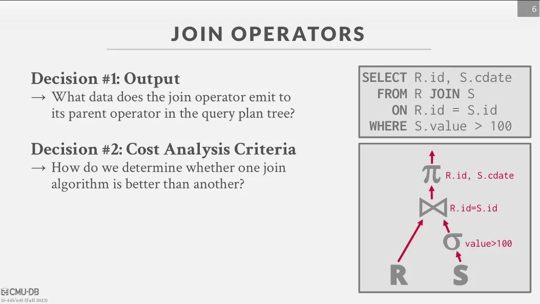
Output
主要有兩種連結方式 :
- Early Materialization : 將所有的資料都放到新的 tuple 中,這樣之後就不需要在回去表中讀取資料,較適合 row store。
- Late Materialization : 只複製 join key 跟 record_id,之後再去表中讀取資料,較適合 column store。
Cost Analysis Criteria
由於資料庫的資料通常無法一次性的讀進記憶體中,因此我們需要透過 join algorithms 來最大化減少硬碟 I/O 的次數,對於 join algorithms 來說,唯一的評論標準就是 I/O 數量。
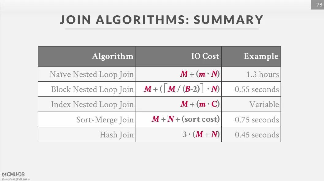
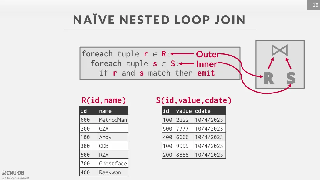
Nested Loop Join
這是最基礎、最直觀的 Join 演算法,就像程式語言中的兩層 for 迴圈。
接下來的資料都是基於以下的假設 :
- 對 跟 兩個 table 做 join
- 有 個 page, 個 tuple
- 有 個 page, 個 tuple
對於以下的 SQL 來說,表 A 是 outer table,表 B 是 inner table。
SELECT *
FROM A
JOIN B ON A.a1 = B.b1;
Naive Nested Loop Join
對於 outer table 的每一個 tuple,都會去 inner table 中掃描全部的 tuple 來進行比對。
Cost 是
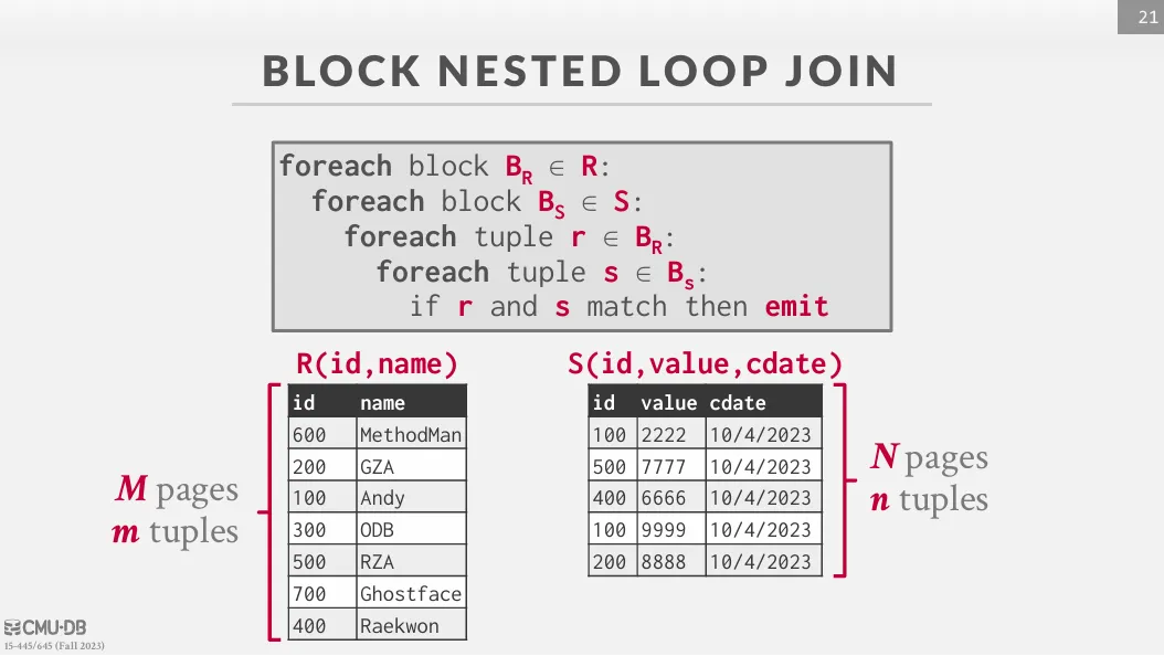
Block Nested Loop Join
每次取 R 的一個 page 進來,然後對 S 掃描全部的 page。
如果我們有 B 塊 buffer,我們可以將一塊用於 inner table 的掃描緩衝,一塊負責輸出,剩下 B - 2 個則用於 outer table。
Cost 的分析如下 :
- 單一 buffer : cost 是
- 有 B 塊 buffer : cost 則變為
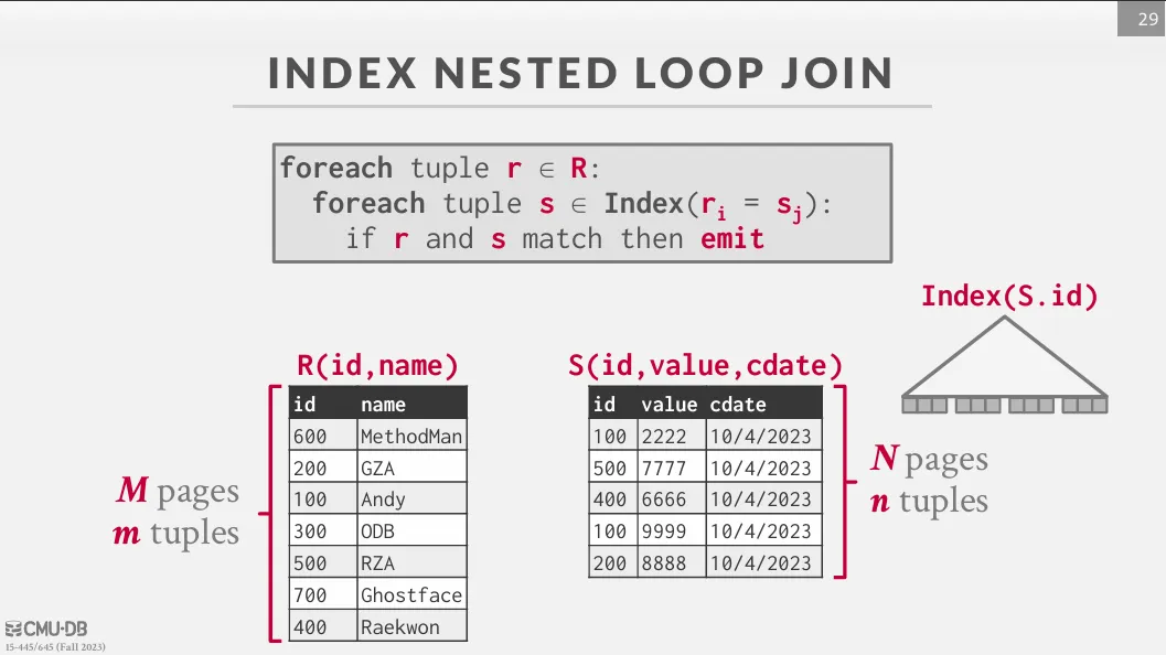
Index Nested Loop Join
前面幾種較慢的原因在於我們需要多次對全表掃描,但若 inner table 在 join attribute 上有 index,我們就可以透過 index 來加速,只需掃描一次即可。
Cost 是 ,其中 C 是掃描一次 index 的 cost。
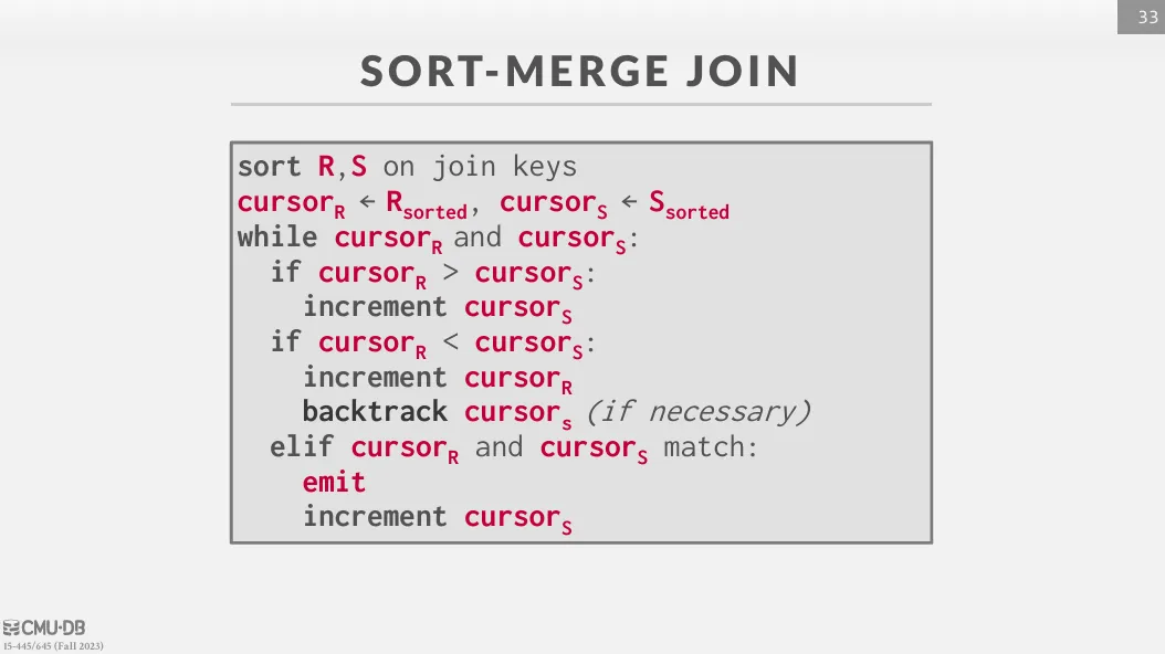
Sort-Merge Join
如果兩個 table 都已經依照 join attribute 排好序了,我們就可以透過 sort-merge join 來進行 join。
主要分為兩個步驟 :
- Sort : 將兩個 table 依照 join attribute 排序
- Merge : 從兩個 table 的端點開始進行掃描,並進行比對,如果遇到重複則需要 backtracking
Cost 的分析如下 :
- Sort cost (R) :
- Sort cost (S) :
- Merge cost :
最差的情況就是所有的 join attribute 都一樣,此時的 cost 是 + sort cost。
Sort merge 主要適用的情境是 :
- 已經有一個或是兩個 table 已經排序好了
- SQL 的輸出必須要排序時
Hash Join
如果有兩個分別在 R 跟 S 的 tuple 有相同的值,則代表他們 hash 之後的值也必定相等,所以我們也可以只針對 hash 之後相同的值進行處理。
Simple Hash Join
這是最基礎的 hash join 方法,如果 outer table 的 hash table 可以放入 memory 中,則可以使用這個方法。
主要分為兩個階段 :
- Build : 將 outer table 中的 join attribute 透過 hash function h1 進行 hash,並放入 hash table T 中 (盡量選擇較小的 table 作為 outer table)
- Probe : 將 inner table 中的 join attribute 透過 hash function h1 得到這個 tuple 在 T 中的位置,並進行比對
其中 T 的 key 是 join attribute,value 則可以是 early materialization 或 late materialization。 在這個方法中,T 有可能沒辦法被放入 memory 中,導致需要進行多次 I/O,如果可以預測 T 的大小,我們也可以使用靜態 hash table。
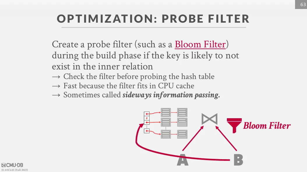
也可以使用 bloom filter 來幫助我們快速找到不在 T 中的 tuple。
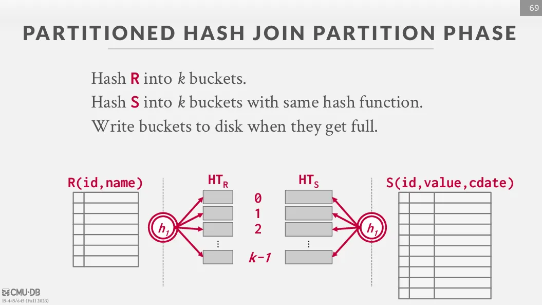
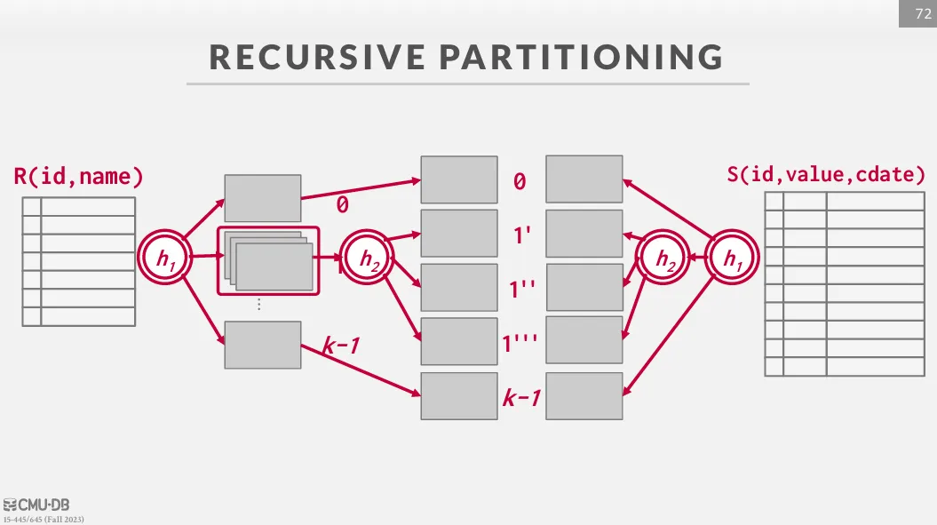
Grace Hash Join / Partitioned Hash Join
如果 hash table 無法放入 memory 中,我們可以使用 Grace Hash Join 來解決這個問題。 這個方法會先將兩個 table 進行 partition,使得每一個 partition 都可以放入 memory 中,然後再對每一組 partition 使用 simple hash join。
主要分為兩個階段 :
- Partition : 將兩個 table 使用同樣的 hash function 進行 partition,使有機會配對成功的 tuple 進入同一個 partition 中
- Probe : 將每一組 partition 中的 tuple 進行 hash join
如果一次 partition 後還是無法放入 memory 中,我們可以進行多次 partition (recursive partitioning),如果單一的 key 有太多的 tuple,可以使用 block nested loop join 來處理。
Cost 的分析如下 :
- partition cost : 讀取之後再寫入到 partition 中
- probe cost : simple hash join 的 cost
- total :
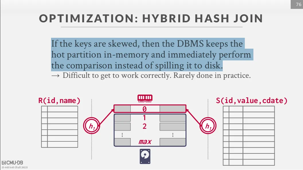
如果有些 key 非常常使用,我們可以將他們放入 memory 中並立即比較,而非溢出到硬碟中。
Conclusion
對於一般的 join 來說,通常都會優先考慮 hash join,除非需要排序 (sort merge join) 或是 inner table 有 index (index nested loop join)。