Sorting & Aggregations Algorithms

這篇筆記會探討資料庫中 Sorting 與 Aggregation 演算法的原理與實作。

Sorting

對於 relational model 來說，它不保證輸出的 tuple 有任何順序關係，但有時候我們需要對結果進行排序，常見的情況如下 :

• ORDER BY
• 使用 DISTINCT 去除重複的 tuple 時
• 當需要大量插入資料到 B+Tree 時，如果有排序就能加快速度
• Aggregations (GROUP BY)

如果資料的大小可以放入記憶體中，我們就可以使用一般的演算法來進行排序 (quick sort / tim sort)，否則我們就必須考慮到 disk I/O 的成本來選擇排序演算法。

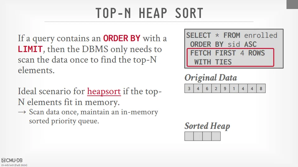
TOP-N Heap Sort

如果我們的 SQL 指令中同時有 LIMIT N 和 ORDER BY 時，我們就可以使用 heap sort 來實現。 這種方法的好處是我們只需要掃一次所有資料並且維護一個大小為 N 的 heap 即可。

TOP-N Heap Sort

External Merge Sort

當資料量大於記憶體時，我們就需要使用外部排序 (external sort) 來處理。

外部排序通常會使用 divide and conquer 的方式來實現，主要包含 2 個步驟 :

• sorting : 將資料分割成小塊，並且在 memory 中進行排序
• merging : 將排序好的資料合併

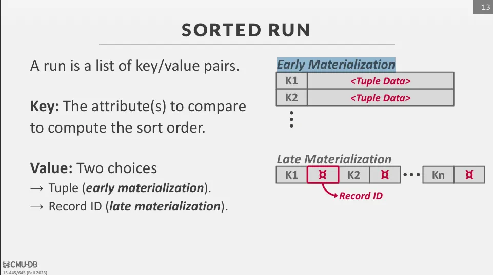
頁面內的排序可以使用 early materialization 或 late materialization 來實現 :

• early materialization : 排序頁面中會儲存完整的資料
• late materialization : 只儲存 record_id 或指標

External Merge Sort

General (K-way) Merge Sort

我們假設 file 被分成 N 個 page，且 DBMS 有 B 個 frame。

第一步 sorting 會將資料分成 $\lceil \frac{N}{B} \rceil$ 個 run，每個 run 的大小為 B page，並且全部載入記憶體中進行排序，接著再將排序好的 run 寫回硬碟。

第二步 merge 就會將這些 run 進行合併，假設我們有 B 個 frame，我們會使用其中一個 frame 作為輸出 buffer，剩下的 B - 1 個 frame 用來存放每個 run 的當前 page。 我們會從每個 run 中取出最小的 tuple，並將其寫入輸出 buffer 中，當輸出 buffer 滿了之後，我們就將其寫回硬碟中，並繼續這個過程直到所有的 run 都被合併完。 在這裡，K-way merge sort 的 K 值為 B - 1。

2-way Merge Sort

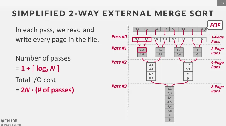
接下來讓我們來計算一下 external merge sort 的 I/O 成本，在處理大量資料時，我們常會用 pass 來表示整個資料被讀取並寫回硬碟的過程，一次 pass 包含兩個 I/O 操作 (讀取與寫回)。

在 sorting 階段，每個 page 都會被讀取並寫回一次，因此成本為一個 pass (2N)。

而在 merge 階段，每一輪都會完整的讀取所有的 page 並寫回，因此成本也是一個 pass (2N)。 我們總共需要執行 $\lceil \log_{B-1} \lceil \frac{N}{B} \rceil \rceil$ 輪的 merge。

因此 external merge sort 的總 I/O 成本為 $1 + \lceil \log_{B-1} \lceil \frac{N}{B} \rceil \rceil$ 個 pass，即 $2N(1 + \lceil \log_{B-1} \lceil \frac{N}{B} \rceil \rceil)$。

External Merge Sort Optimizations

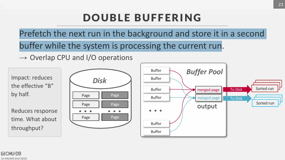
Double Buffering Optimization

在 merge 階段，我們可以使用 double buffering 來減少等待 I/O 的時間。

當一個 buffer 正在被寫回硬碟時，另一個 buffer 可以繼續被填滿，這樣就能減少等待時間。

Double Buffering

Comparison Optimizations

Code Specialization

通用的排序函數通常接受一個函數指標 (Function Pointer) 或 callback 作為比較器，例如 C++ std::sort 的 Compare 參數。 每次比較，CPU 都需要透過函數指標進行一次間接呼叫 (Indirect Call)。這會打斷 CPU 的指令管線 (instruction pipeline)，並可能導致分支預測失敗，效能較差。 因此我們可以將函數指標內聯 (inline) 到排序函數中，這樣就能減少間接呼叫的次數，提升效能。

Suffix Truncation

如果排序的是長字串 (VARCHAR)，我們可以只比較字串的前幾個字元，這樣就能減少比較的次數，提升效能。

Using B+tree

如果已經有 B+tree 的索引，我們只需要使用 B+tree 來快速遍歷 leaf node 即可得到排序好的資料，但會分成兩種情況 :

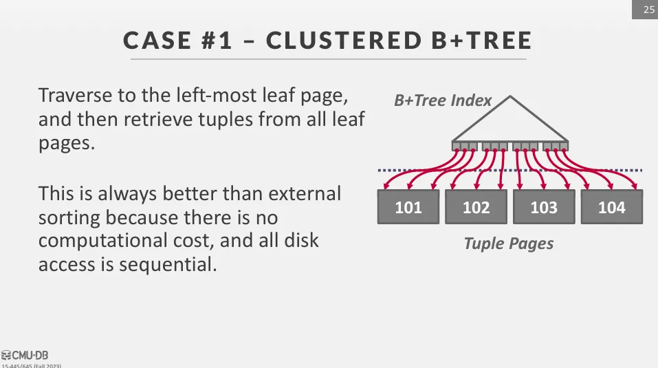
Clustered B+tree

I/O 是有順序的，比外部排序效率更高

Clustered B+tree

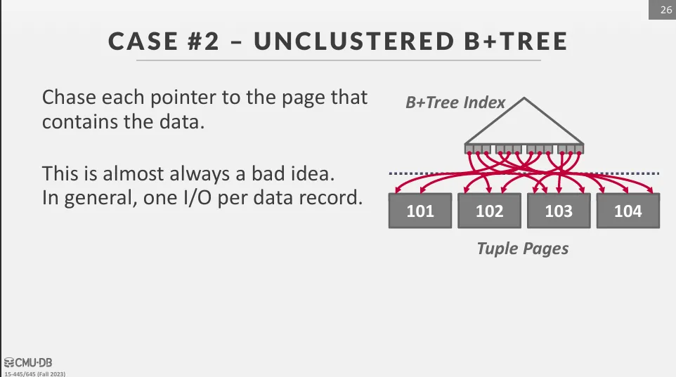
Unclustered B+tree

I/O 是隨機的，效率極低

Unclustered B+tree

Aggregations

為了將多個 tuple 的單個屬性合併成一個值，DBMS 需要能將資料快速分組的方法。

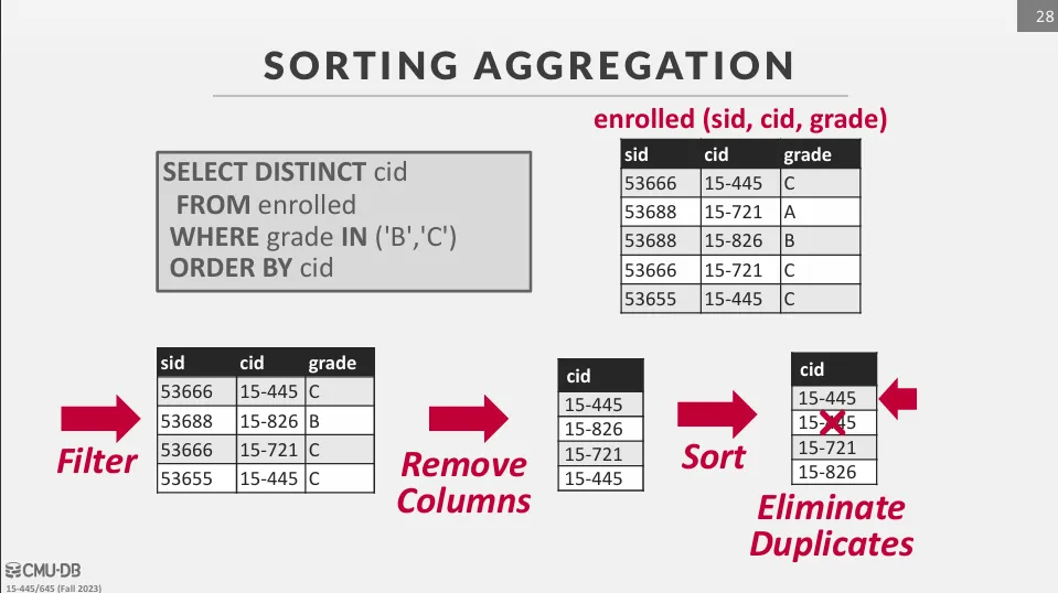
Sorting

將資料依照 grouping key 排序，然後進行聚合，這種方法的好處是可以利用排序的結果來加速聚合運算，但缺點是排序的成本較高，特別是當資料量大於記憶體時。

如下圖的範例，由於我們使用了 DISTINCT，因此我們需要先將資料排序，接著再進行聚合。

Sorting

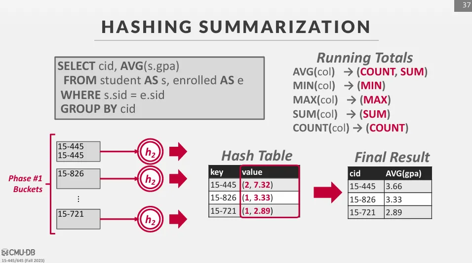
Hashing

如果我們不需要最後輸出的結果是排序的，我們可以使用 hashing 來進行聚合。 這種方法的好處是可以在一次掃描中完成聚合運算，缺點是需要額外的記憶體來存放 hash table。

使用這種方式會有兩個階段 :

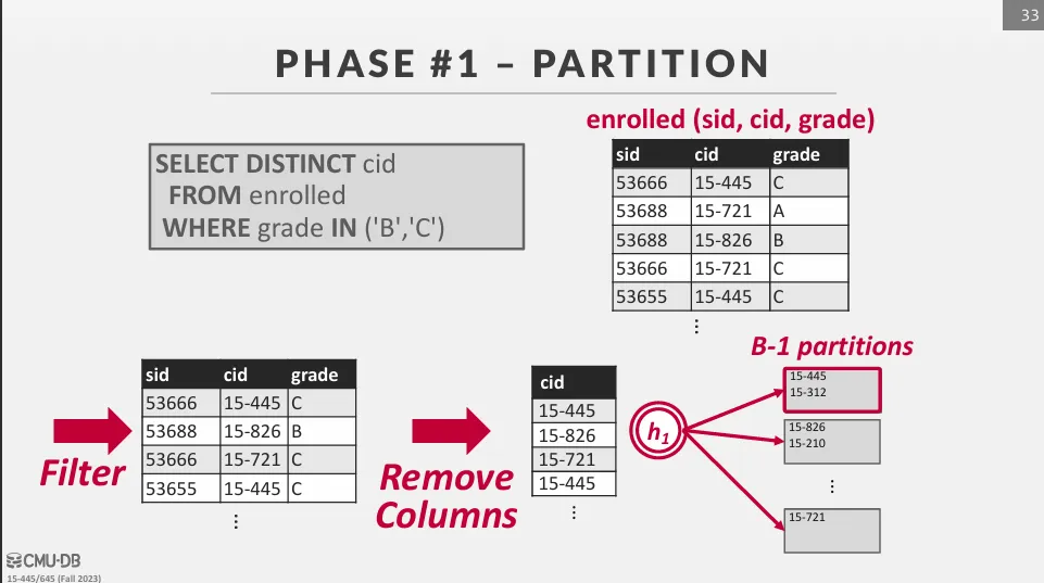
Phase 1 : Partition

先將一個巨大的資料集分割成多個較小的 partition，並保證相同的 grouping key 會被分配到同一個 partition 中。

如果我們總共有 B 個 frame 可以使用，使用 hash function h1 來將 tuple 分配到 B - 1 個 partition 中，剩下的一個 partition 用來存放輸入的資料。

Partition

Phase 2 : ReHash

把每個 partition 都逐一讀到記憶體裡，並使用 hash function h2 來建立一個新的 hash table 來進行聚合運算。 這裡不使用同一個 hash function 的原因是為了避免資料傾斜，如果 h1 已經把大量不同的鍵值分配到同一個 partition 中，我們會希望 h2 能將這些鍵值均勻地分配到 hash table 中。

ReHash

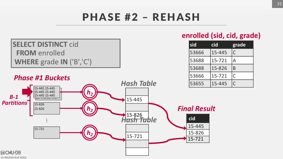
在 rehash 的過程中，存在一組 grouping key -> return value 的 hash table，我們只需要更新這個 key-value pair 即可。

ReHash